GEARS - Geospatial Ecology and Remote Sensing lab - https://www.geospatialecology.com

Introduction to Remote Sensing of the Environment

Lab 5 - Image Classification - part 2

Acknowledgments

• Google Earth Engine Team
• Google Earth Engine Developers group

---

Prerequisites

---

Completion of this lab exercise requires use of the Google Chrome browser and a Google Earth Engine account. If you have not yet signed up - please do so now in a new tab:

Earth Engine account registration

Once registered you can access the Earth Engine environment here: https://code.earthengine.google.com

This lab follows on from others (Introductory Remote Sensing Labs 1-4) in this series.

---

Objective

The objective of this lab is to further your understanding of the image classification process, and improve the classification from last week.

---

Load up your previous classification from last week

Open you script from last week's lab. If you did not save it, repeat the steps from IRS Lab 4 and be sure to save it this time.

I have provided the full code below, but remember that you need to manually collect the training data and assign landcover properties.

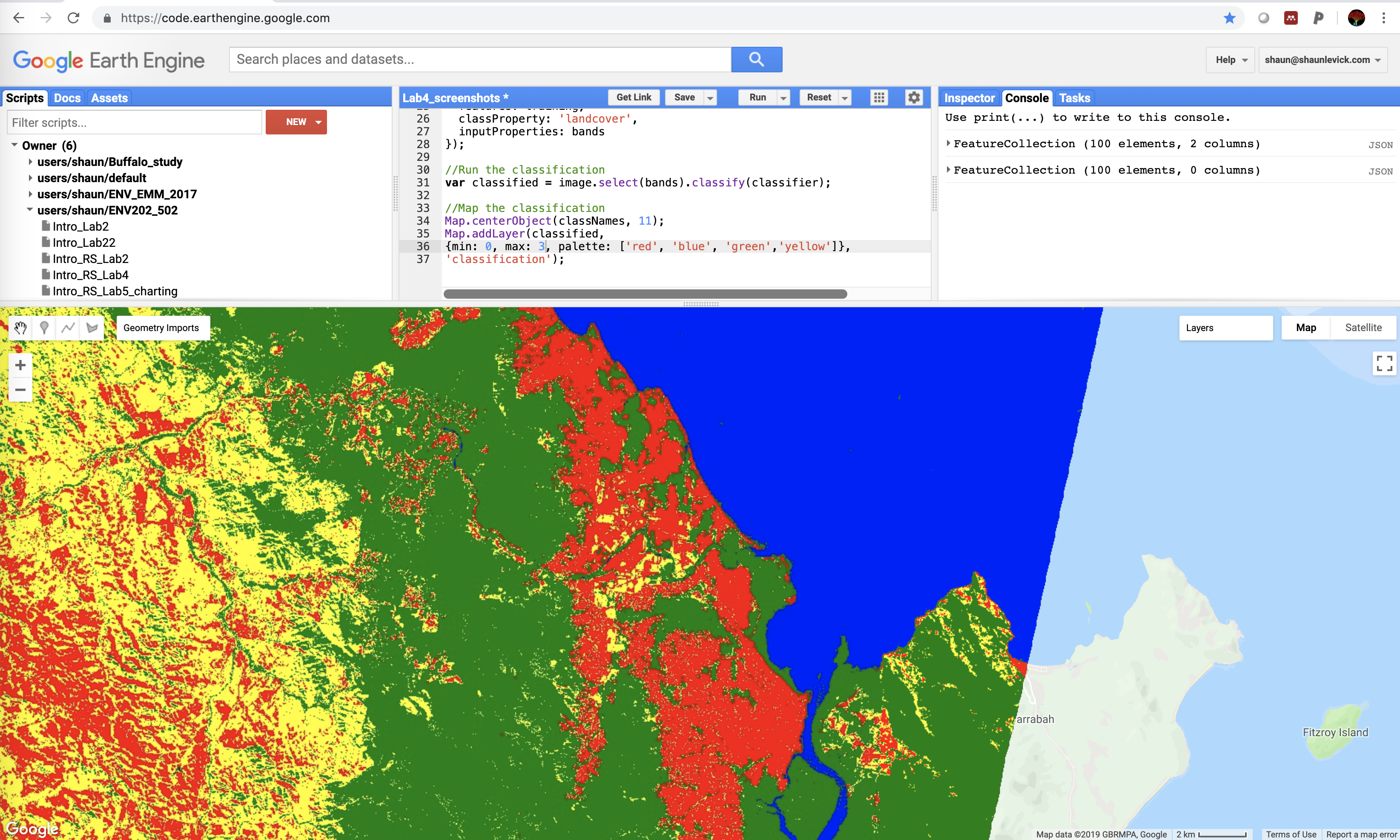
//Filter image collection for time window, spatial location, and cloud cover
var image = ee.Image(ee.ImageCollection('LANDSAT/LC08/C01/T1_SR')
    .filterBounds(roi)
    .filterDate('2016-05-01', '2016-06-30')
    .sort('CLOUD_COVER')
    .first());

//Add true-clour composite to map
Map.addLayer(image, {bands: ['B4', 'B3', 'B2'],min:0, max: 3000}, 'True colour image');

//Merge features into one FeatureCollection
var classNames = urban.merge(water).merge(forest).merge(agriculture);

//Select bands to use
var bands = ['B2', 'B3', 'B4', 'B5', 'B6', 'B7'];

//Sample the reflectance values for each training point
var training = image.select(bands).sampleRegions({
  collection: classNames,
  properties: ['landcover'],
  scale: 30
});

//Train the classifier - in this case using a CART regression tree
var classifier = ee.Classifier.cart().train({
  features: training,
  classProperty: 'landcover',
  inputProperties: bands
});

//Run the classification
var classified = image.select(bands).classify(classifier);

//Display the classification map
Map.centerObject(classNames, 11);
Map.addLayer(classified,
{min: 0, max: 3, palette: ['red', 'blue', 'green','yellow']},
'classification');

---

Improving the Classification

We ended last week with a discussion on whether or not we were happy with this classification. Even without any quantitative data, it was clearly lacking in some regions. How can we improve it? There are a few option we can explore:

1. Change the training sample size. We only sampled 25 pixels per class. This was a lot of clicking, but we could use polygons instead of points to sample more pixels for training.
2. Change the sampling strategy. We collected an even number of points per class, but some landcover class cover much more area than others. We could experiment with a stratified sampling approach instead.
3. Change the classifier. We used a CART classifier, we could try a different approach such as a support vector machine (SVM) or randomForest (randomForest) approach.
4. Change the bands. We could add ancillary information, such as elevation data, or a derived index such as NDVI to provide for information for class discrimination.
5. Change the image. We used a winter scene from Landsat-8. We could try a summer scene, or switch to a Sentinel-2 image.

---

Thank you

I hope you found that useful. A recorded video of this tutorial can be found on my YouTube Channel's Introduction to Remote Sensing of the Environment Playlist and on my lab website GEARS.

Kind regards, Shaun R Levick

---