![]() https://www.geospatialecology.com
https://www.geospatialecology.com
Environmental Monitoring and Modelling
Lab 2 - Getting deeper into Earth Engine
Objective
In Lab 1 we learnt how to search for a single image and display it in the map environment. From an environmental monitoring perspective we will often be interested in how and where landscapes, and different components of that landscape, change over time. Understanding landscape context is very important, as ecological processes change with topographic position. In this lab we will learn how to access, visualise and query digital elevation data for any study location.
Acknowledgments
- Google Earth Engine Team
- Geospatial Analysis Lab, University of San Francisco (especially Nicholas Clinton and David Saah)
The Earth Engine Interface
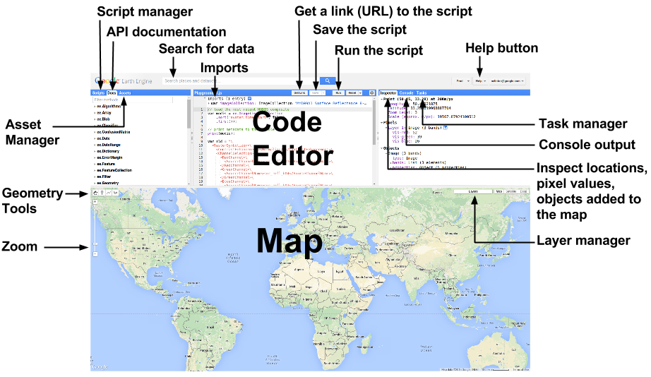
- Editor Panel
- The Editor Panel is where you write and edit your Javascript code
- Right Panel
- Console tab for printing output.
- Inspector tab for querying map results.
- Tasks tab for managing long running tasks.
- Left Panel
- Scripts tab for managing your programming scripts.
- Docs tab for accessing documentation of Earth Engine objects and methods, as well as a few specific to the Code Editor application
- Assets tab for managing assets that you upload.
- Interactive Map
- For visualising map layer output
- Search Bar
- For finding datasets and places of interest
- Help Menu
- User guide reference documentation
- Help forum Google group for discussing Earth Engine
- Shortcuts Keyboard shortcuts for the Code Editor
- Feature Tour overview of the Code Editor
- Feedback for sending feedback on the Code Editor
- Suggest a dataset. Our intention is to continue to collect datasets in our public archive and make them more accessible, so we appreciate suggestions on which new datasets we should ingest into the Earth Engine public archive.
Getting started with elevation data
- Clear the script by selecting "Clear script" from the Reset button dropdown menu.
- Search for “elevation” and click on the SRTM Digital Elevation Data 30m result to show the dataset description.
- Click on Import, which moves the variable to the Imports section at the top of your script. Rename the default variable name "image" to be "srtm".
- Add the image object to the map with the script:
print(srtm);
- Browse through the information that was printed. Open the “bands” section to show the one band named “elevation”. Note that all this same information is automatically available for all variables in the Imports section.
- Use the Map.addLayer() method to add the image to the interactive map. We will start simple, without using any of the optional parameters.
Map.addLayer(srtm);
The displayed map will look pretty flat grey, because the default visualization parameters map the full 16bit range of the data onto the black–white range, but the elevation range is much smaller than that in any particular location. We’ll fix it in a moment.
- Select the Inspector tab. Then click on a few points on the map to get a feel for the elevation in this area. Finally, set visualization parameters:
Map.addLayer(srtm, {min: 0, max: 1000}, 'DEM');
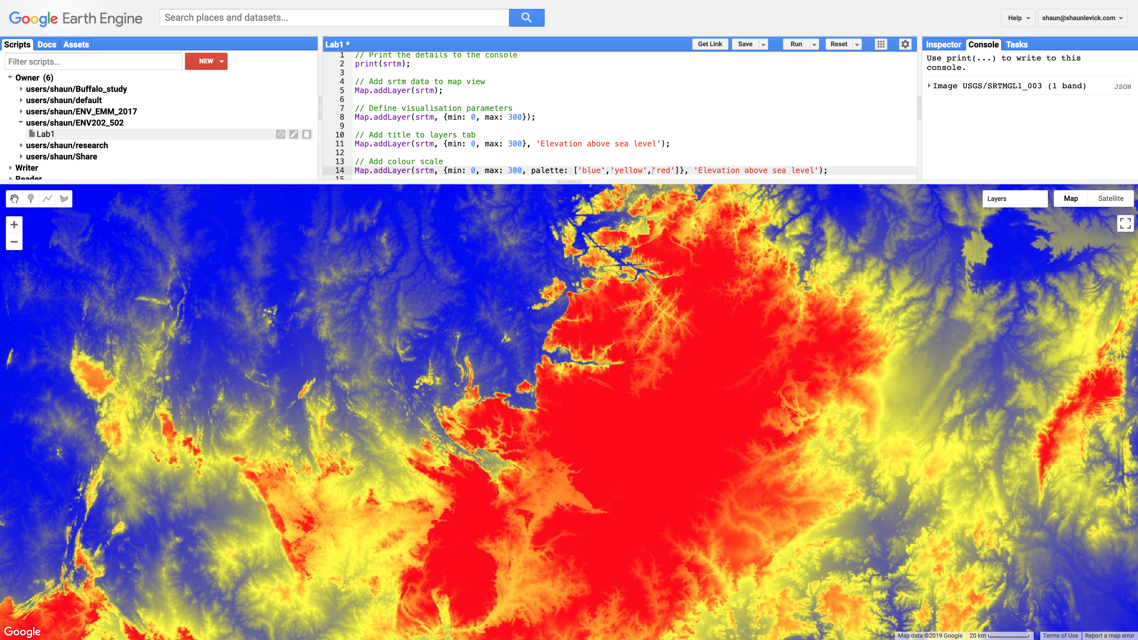
- If you would like to experiment with different colour combinations, you can play with colour palettes as per the example below:
Map.addLayer(srtm, {min: 0, max: 300, palette: ['blue', 'yellow', 'red']}, 'Elevation above sea level');
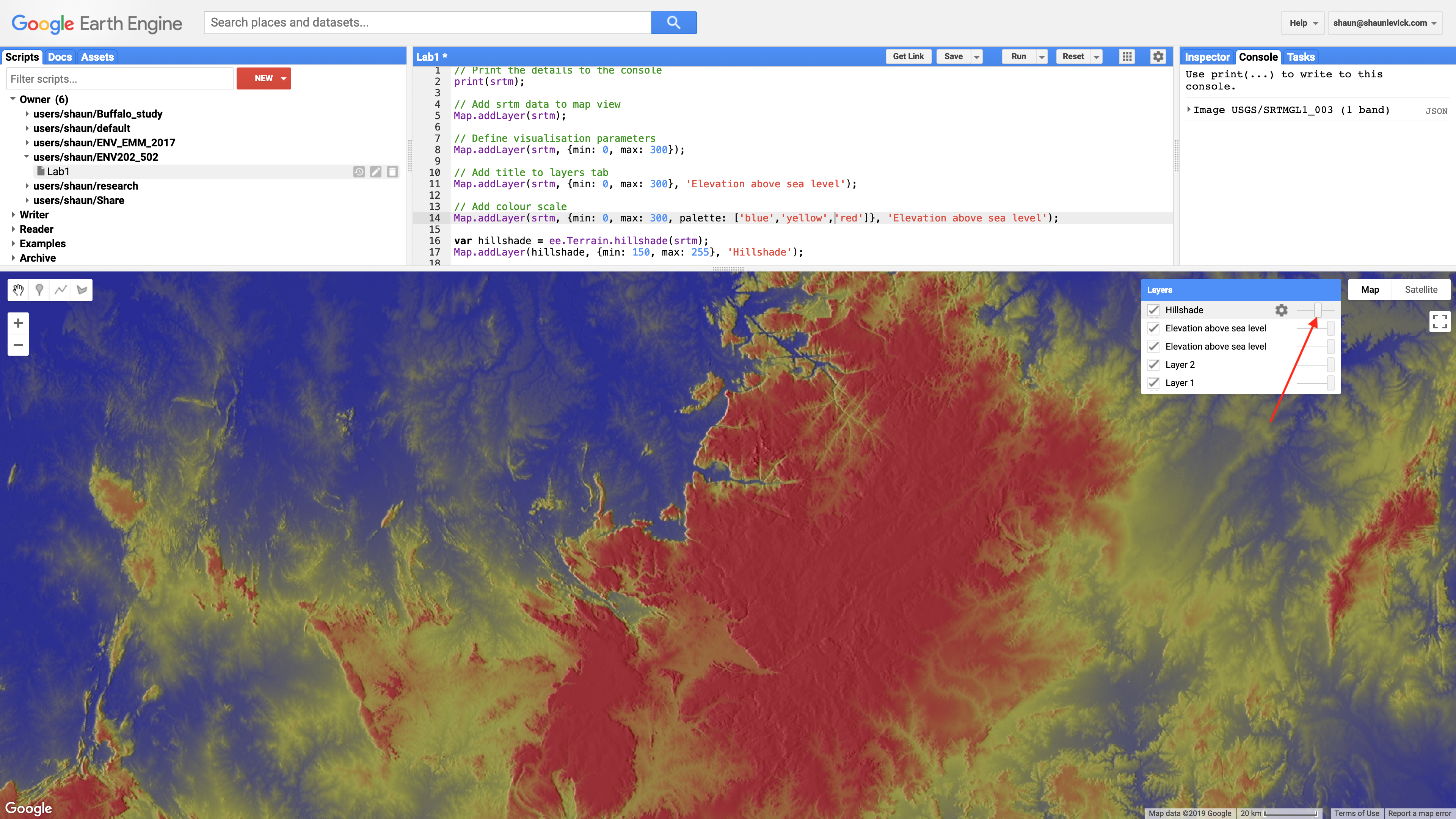
Hillshading and slope
- For better visualisation we can create a hillshade view of the elevation data. Remember you can use the Layer transparency options to create draped images for colourised hillshades.
var hillshade = ee.Terrain.hillshade(srtm);
Map.addLayer(hillshade, {min: 150, max:255}, 'Hillshade');
Applying a computation to an image
- Pan over to the Kakadu National Park region, where there are some nice elevation differences.
- Next add a simple computation, for example a threshold on elevation.
var high = srtm.gt(200);
Map.addLayer(high, {}, 'Above 200m');
- Do another computation to compute slope from the elevation data and display it on the map as a separate layer. Also add a third parameter to the addLayer() method, which names the layer.
var slope = ee.Terrain.slope(srtm);
Map.addLayer(slope, {min: 0, max: 60}, 'Slope');
Apply a spatial reducer
- Select the polygon geometry tool and draw a triangle (or more complex polygon) on the map.
- Print the mean value for the region.
Map.addLayer(srtm, {min: 0, max: 1000}, 'DEM');
Map.addLayer(geometry);
var dict = srtm.reduceRegion({
        reducer: 'mean',
        geometry: geometry,
        scale: 90
});
print('Mean elevation', dict);
- Clear the workspace by clicking Reset > Clear script
GEARS - Geospatial Ecology and Remote Sensing lab - https://www.geospatialecology.com (c) Shaun R Levick