GEARS - Geospatial Ecology and Remote Sensing lab - https://www.geospatialecology.com

Introduction to Remote Sensing of the Environment

Lab 1 - Getting started with Google Earth Engine

---

Acknowledgments

• Google Earth Engine Team
• Earth Engine Beginning Curriculum

---

Prerequisites

---

Completion of this lab exercise requires use of the Google Chrome browser and a Google Earth Engine account. If you have not yet signed up - please do so now in a new tab:

Earth Engine account registration

Once registered you can access the Earth Engine environment here: https://code.earthengine.google.com

Google Earth Engine uses the JavaScript programming language. We will cover the very basics of this language during this course. If you would like more detail you can read through the introduction provided here:

JavaScript background

---

Objective

---

The objective of this lab is to give you an introduction to the Google Earth Engine processing environment. By the end of this exercise you will be able to search, find and visualise a broad range of remotely sensed datasets. We will start with single-band imagery - elevation data from the SRTM mission.

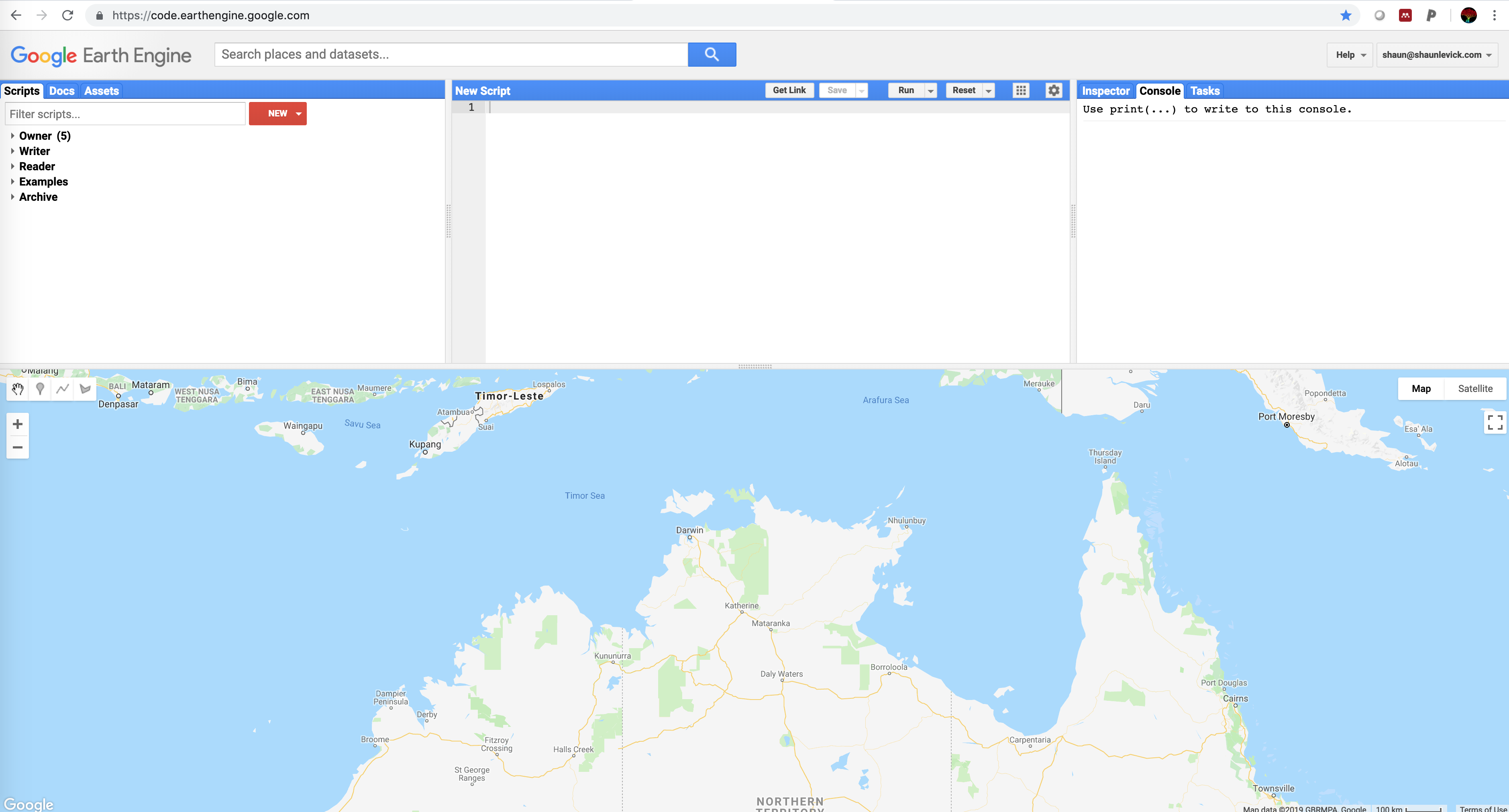
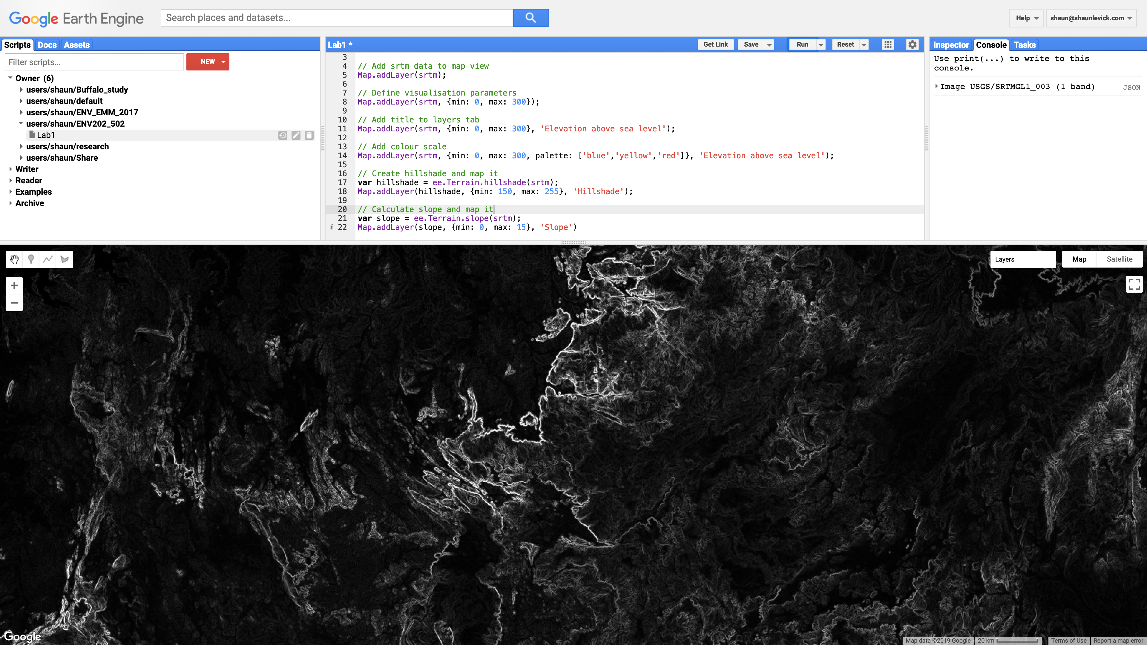
1. The Earth Engine code editor

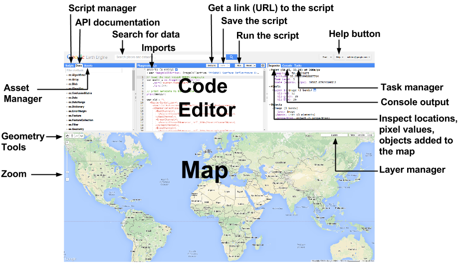
1. Editor Panel
   • The Editor Panel is where you write and edit your Javascript code
2. Right Panel
   • Console tab for printing output.
   • Inspector tab for querying map results.
   • Tasks tab for managing long­ running tasks.
3. Left Panel
   • Scripts tab for managing your programming scripts.
   • Docs tab for accessing documentation of Earth Engine objects and methods, as well as a few specific to the Code Editor application
   • Assets tab for managing assets that you upload.
4. Interactive Map
   • For visualizing map layer output
5. Search Bar
   • For finding datasets and places of interest
6. Help Menu
   • User guide ­ reference documentation
   • Help forum ­ Google group for discussing Earth Engine
   • Shortcuts ­ Keyboard shortcuts for the Code Editor
   • Feature Tour ­ overview of the Code Editor
   • Feedback ­ for sending feedback on the Code Editor
   • Suggest a dataset. Our intention is to continue to collect datasets in our public archive and make them more accessible, so we appreciate suggestions on which new datasets we should ingest into the Earth Engine public archive.

---

2. Getting started with images

• Navigate to Darwin and zoom in using the mouse wheel.

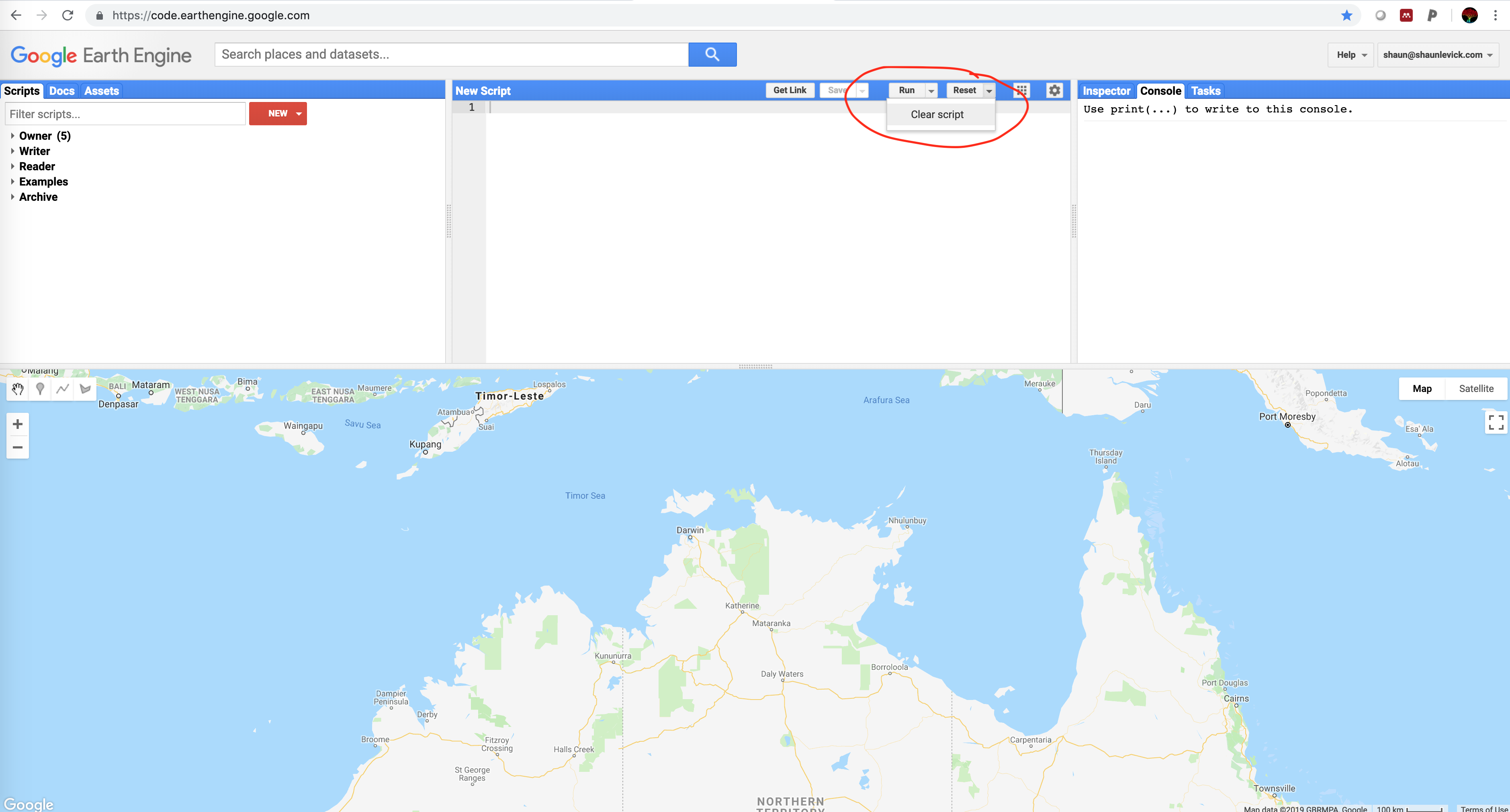
• Clear the script workspace by selecting "Clear script" from the Reset button dropdown menu.

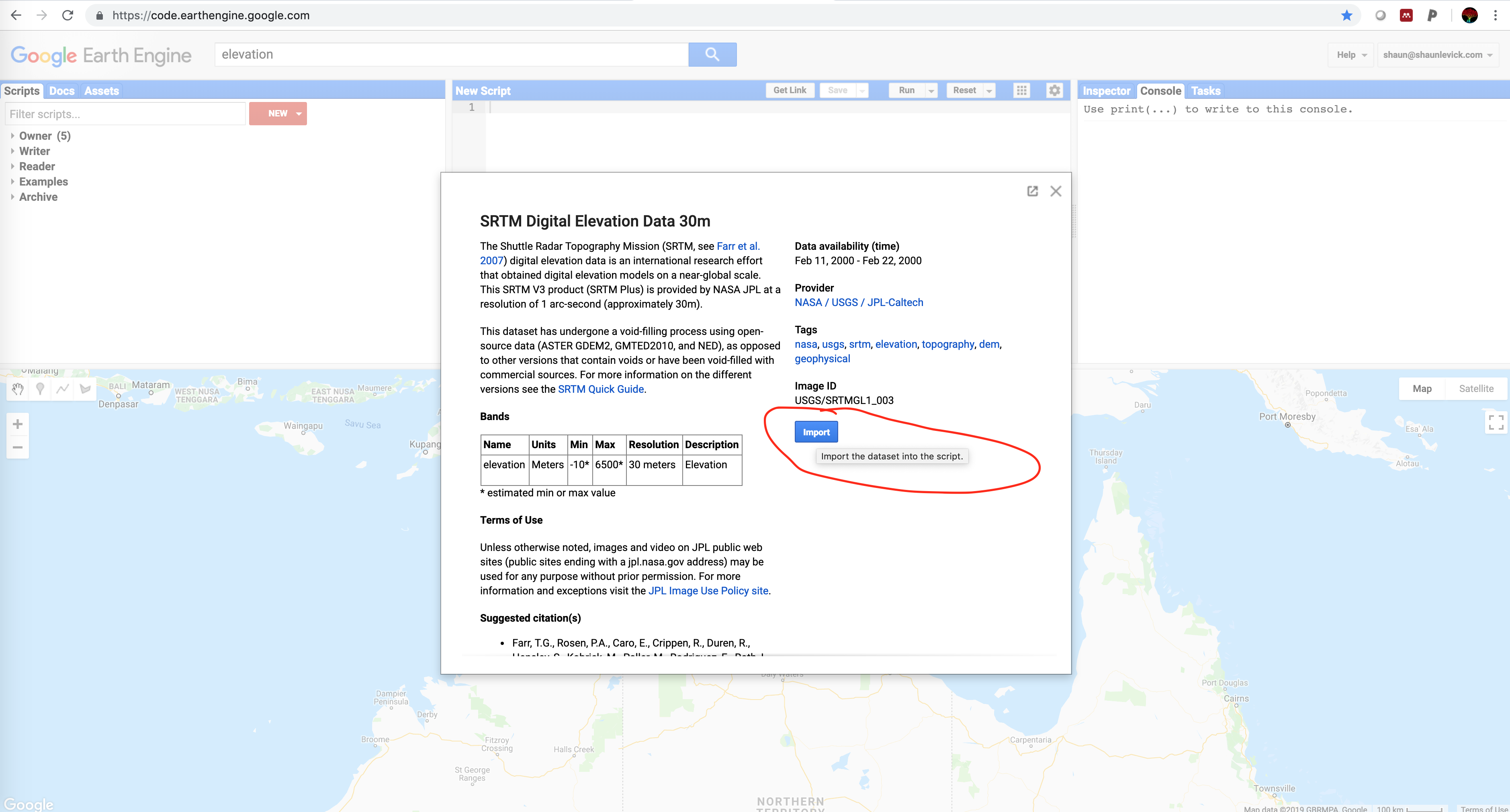
• Search for “elevation” and click on the SRTM Digital Elevation Data 30m result to show the dataset description.

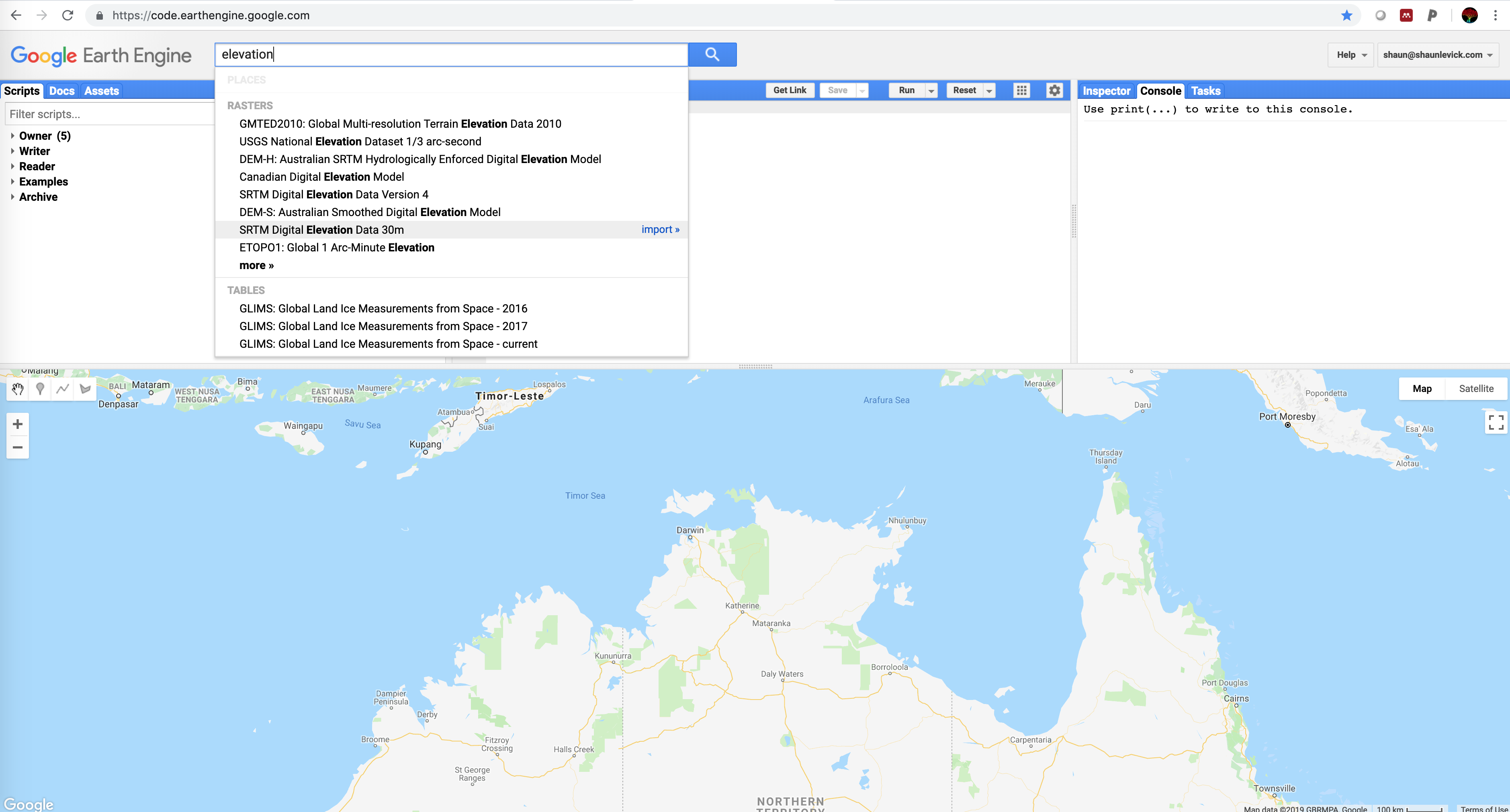
• View the information on the dataset, and then click on Import, which moves the variable to the Imports section at the top of your script.

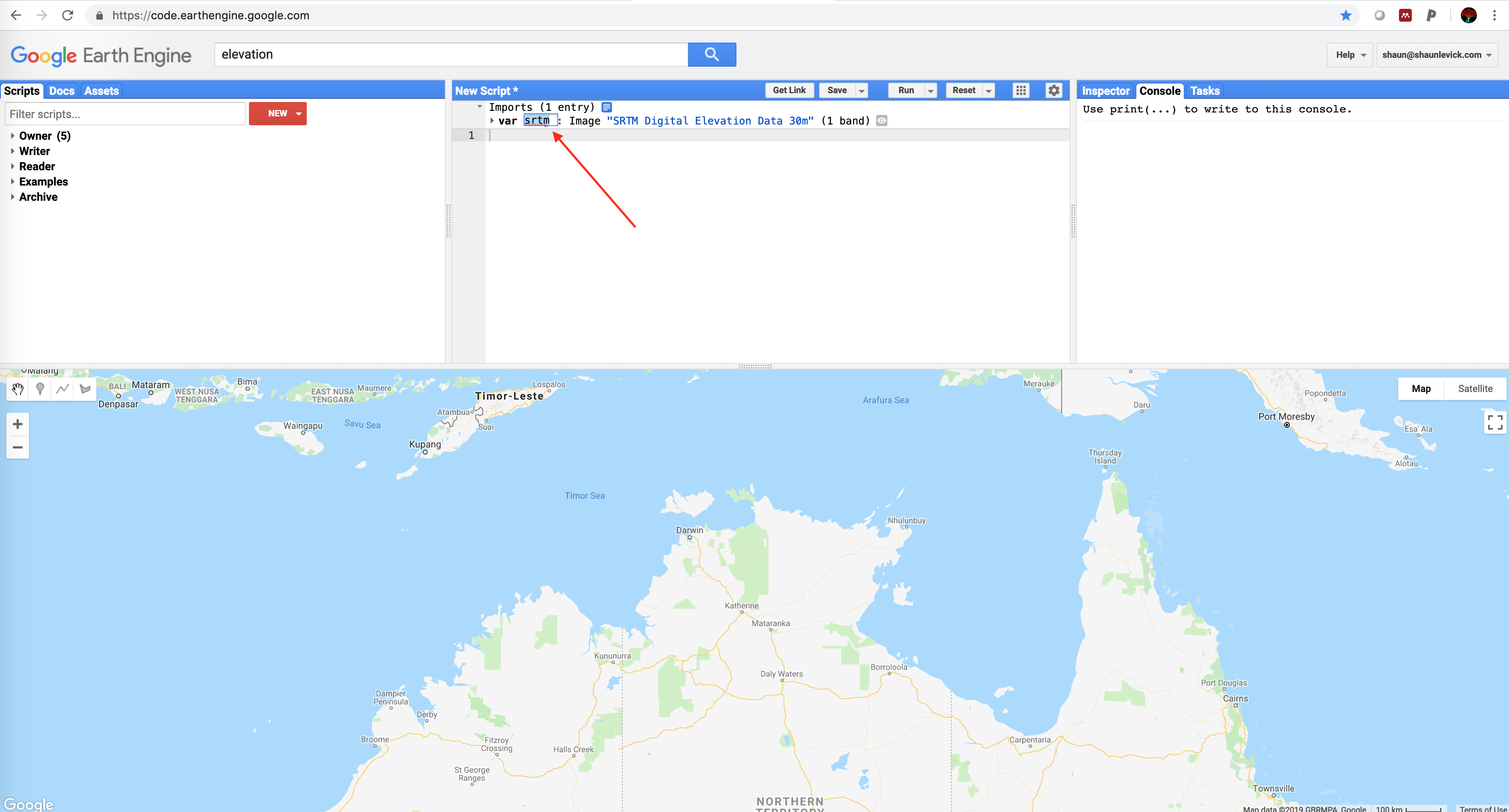
• Rename the default variable name "image" to be "srtm".

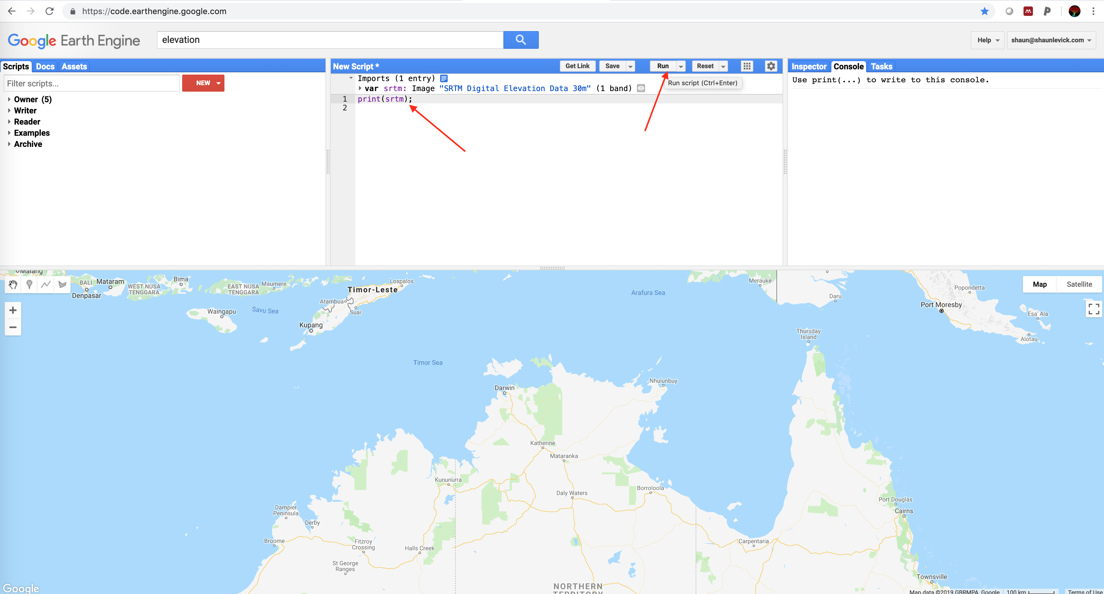
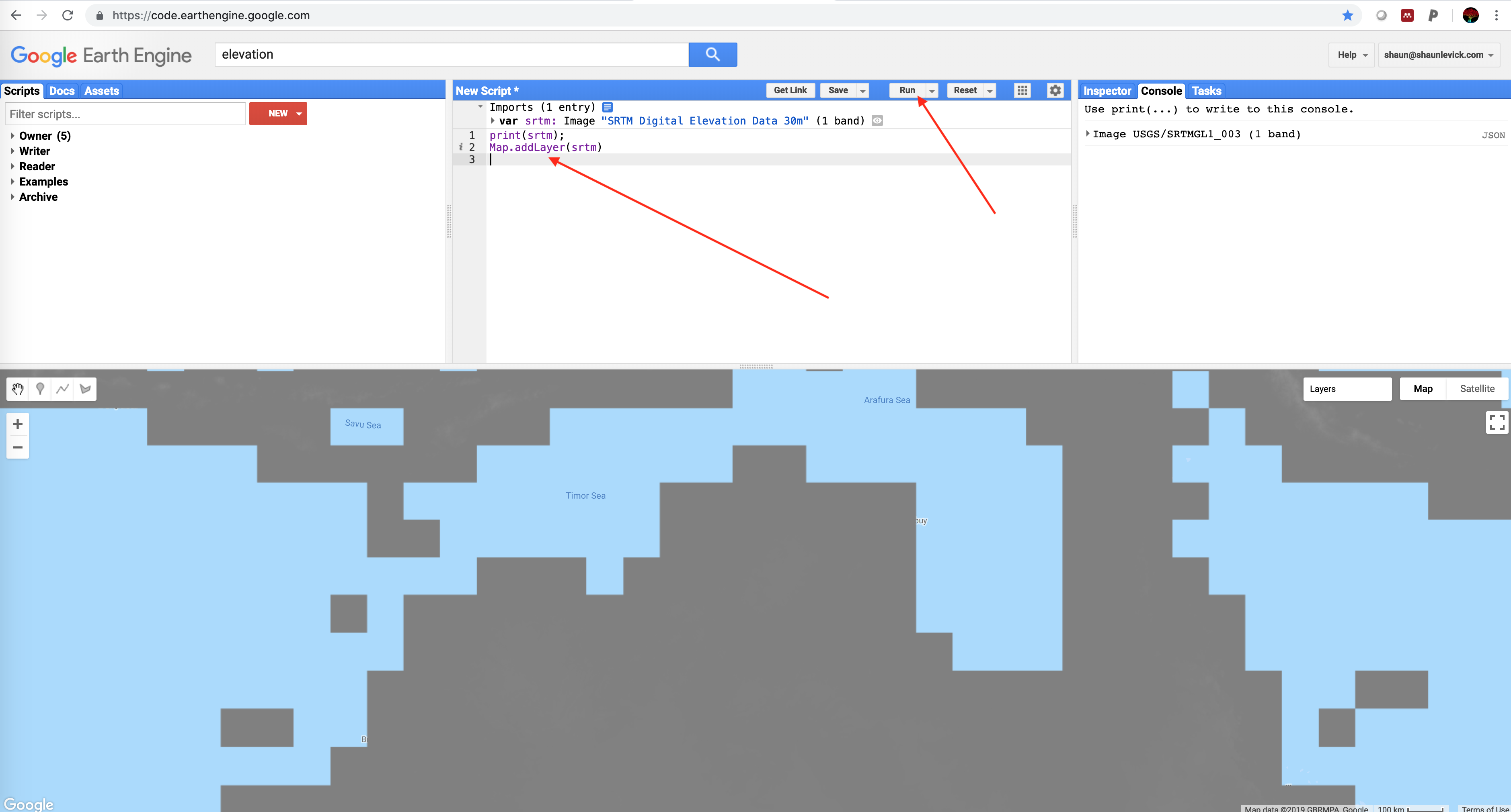
• Add the image object to the console by coping the script below into the code editor, and click "run" :

print(srtm);

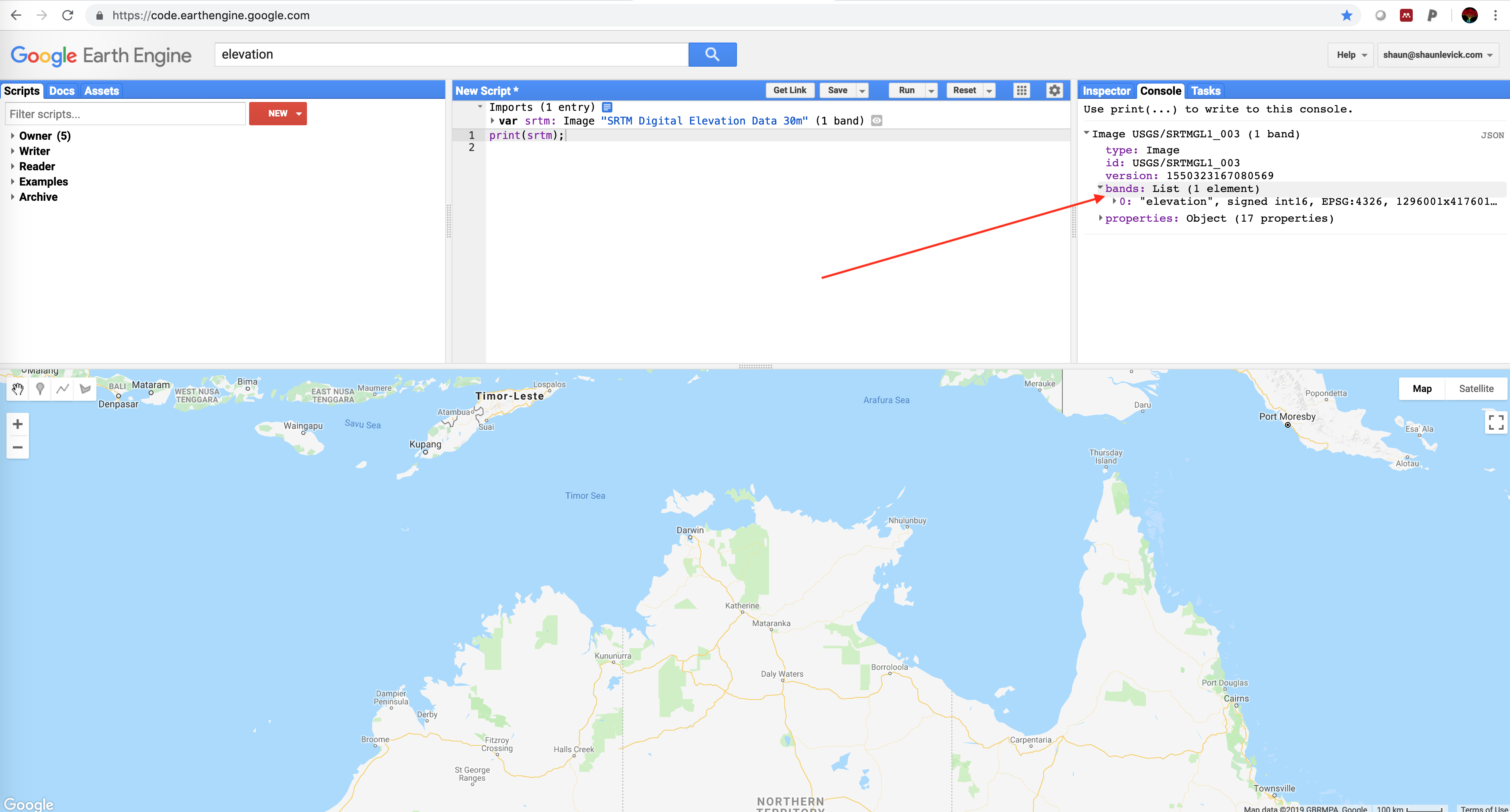
• Browse through the information that was printed to the console. Open the “bands” section to show the one band named “elevation”. Note that all this same information is automatically available for all variables in the Imports section.

• Use the Map.addLayer() method to add the image to the interactive map. We will start simple, without using any of the optional parameters.

Map.addLayer(srtm);

Adjusting visualisation parameters

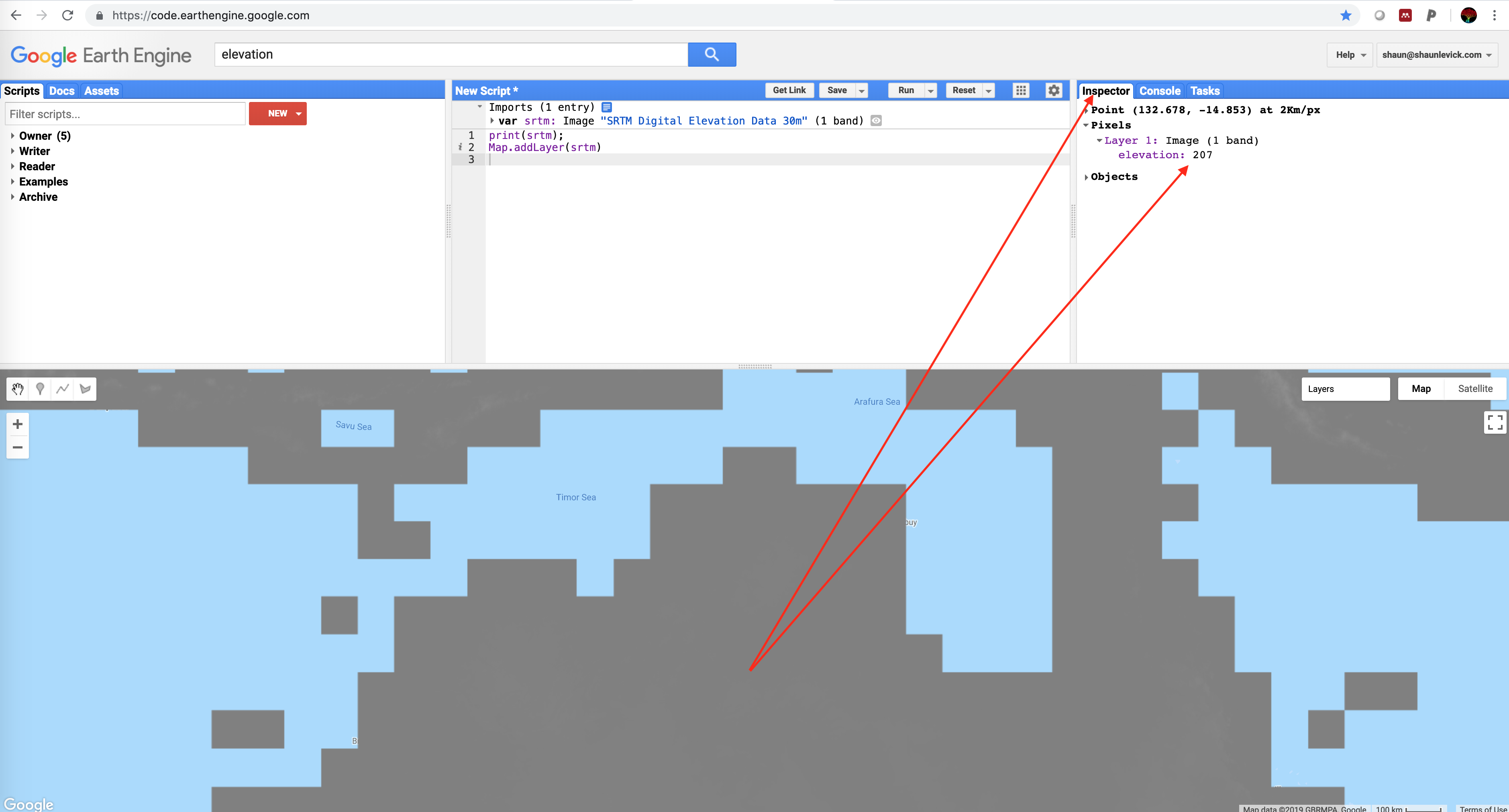
The displayed map will look pretty flat grey, because the default visualization parameters map the full 16­bit range of the data onto the black–white range, but the elevation range is much smaller than that in any particular location. We’ll fix it in a moment.

• Select the Inspector tab. Then click on a few points on the map to get a feel for the elevation range in this area.

• Now you can set some more appropriate visualization parameters by adjusting the code as follows (units are in meters above sea level):

Map.addLayer(srtm, {min: 0, max: 300});

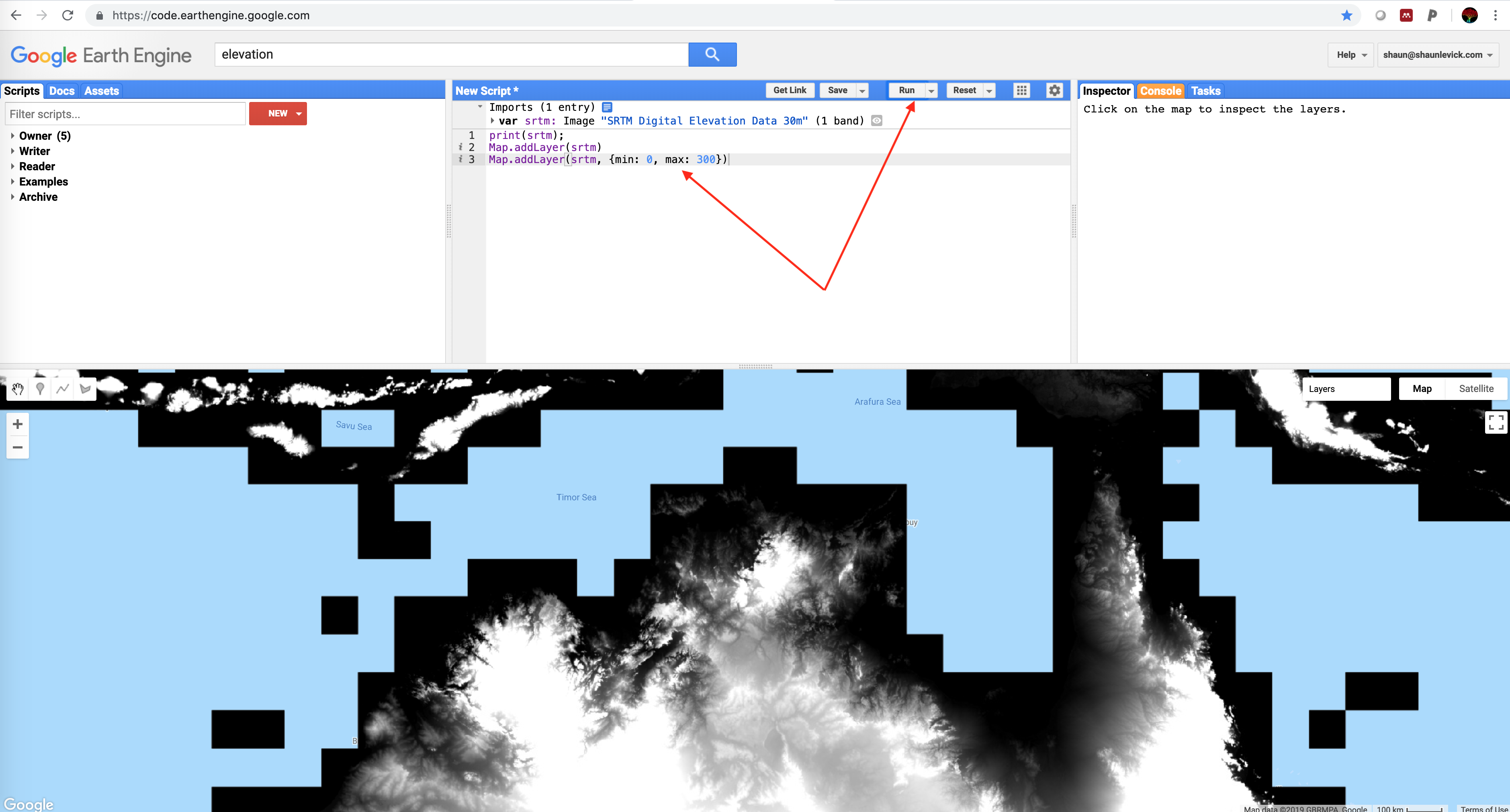
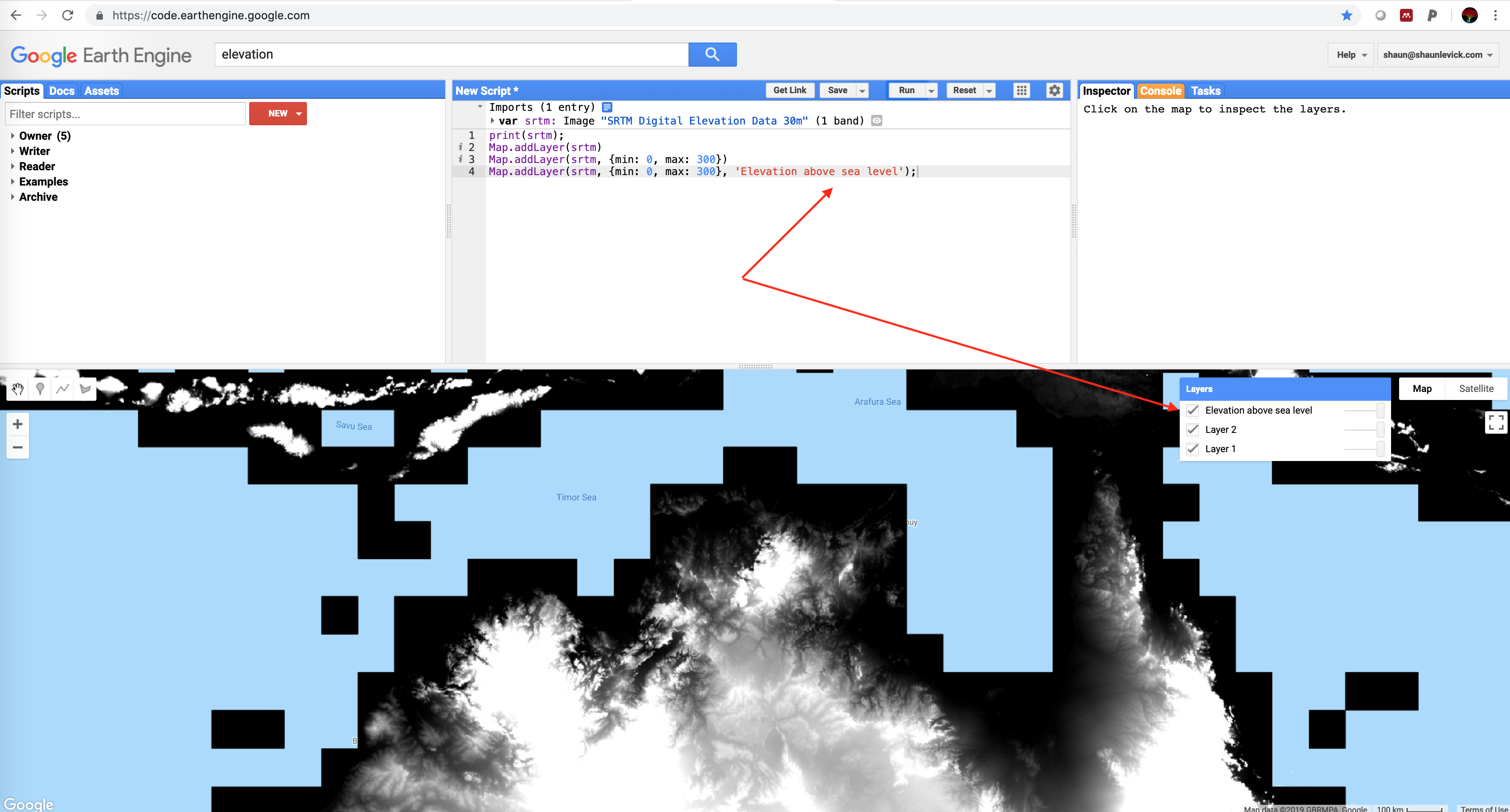
• You will now be able to see variation in elevation range with low values in black and highest points in white. Layers added to the map will have default names like "Layer 1", "Layer 2", etc. To improve the readability, we can give each layer a human­-readable name, by adding a title with the syntax in the following code. Don't forget to click run.

Map.addLayer(srtm, {min: 0, max: 300}, 'Elevation above sea level');

Commenting and saving your scripts

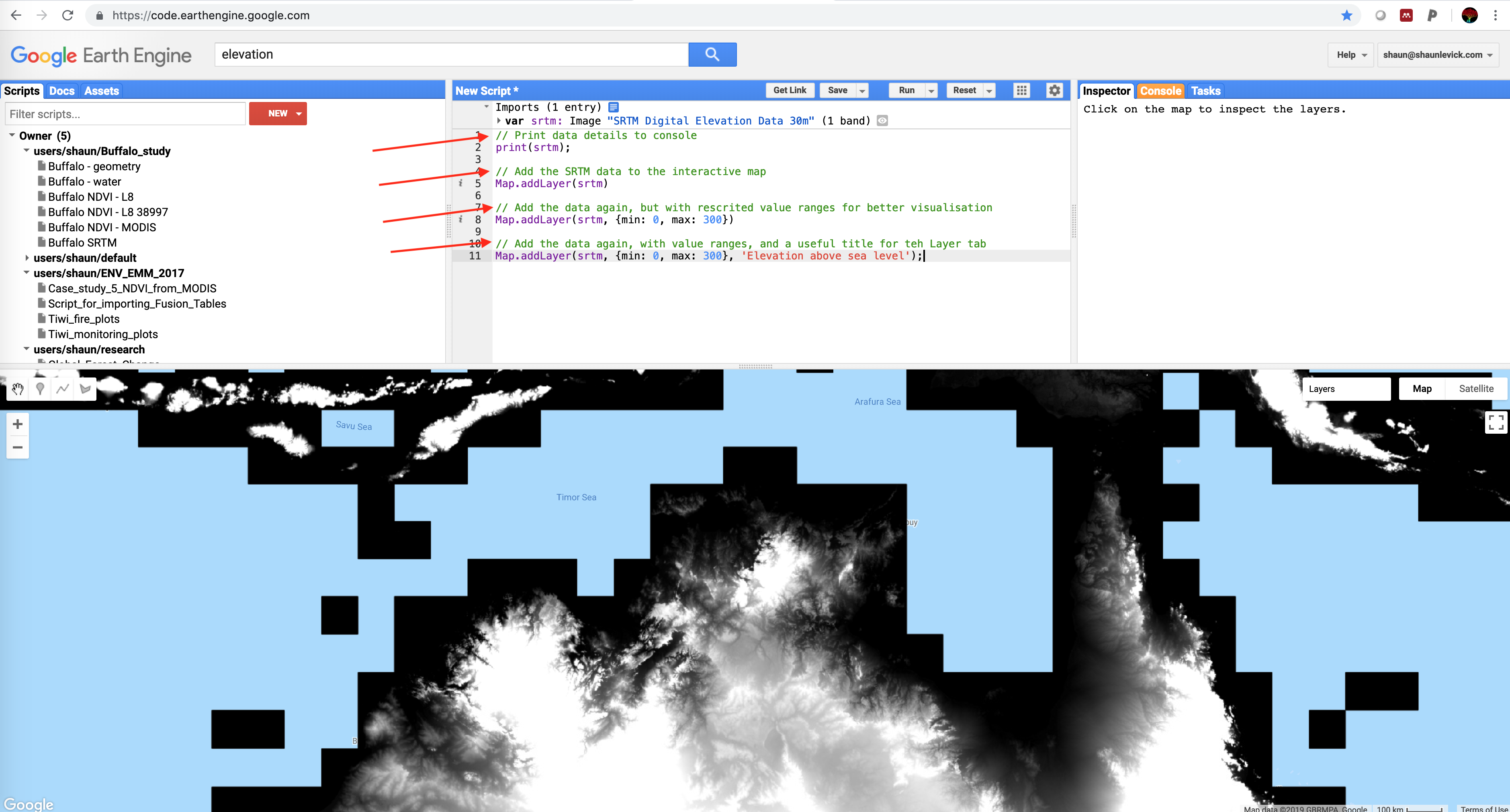
• Now the last step for today is to save your code, however before doing that it is good practice to add a some comment lines to your code reminding you of what you did and why. We add these with two forward slashes // :

// Print data details to console
print(srtm);

// Add the SRTM data to the interactive map
Map.addLayer(srtm)

// Add the data again, but with rescrited value ranges for better visualisation
Map.addLayer(srtm, {min: 0, max: 300})

// Add the data again, with value ranges, and a useful title for teh Layer tab
Map.addLayer(srtm, {min: 0, max: 300}, 'Elevation above sea level');

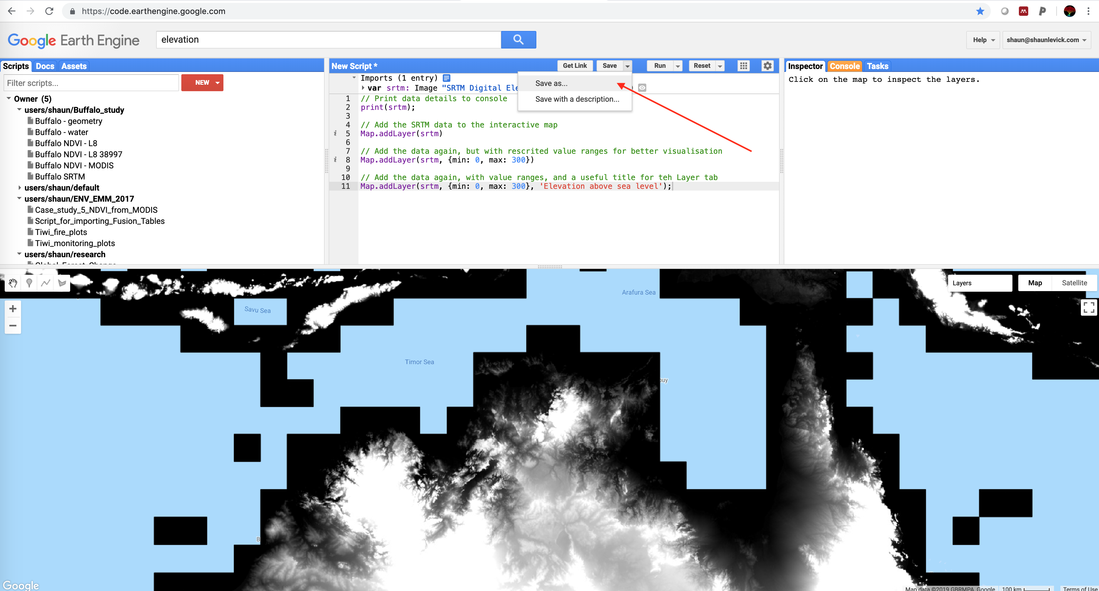
• The next step is then to save you script by clicking "Save". It will be saved in your private repository, and will be accessible the next time you log in to Earth Engine.

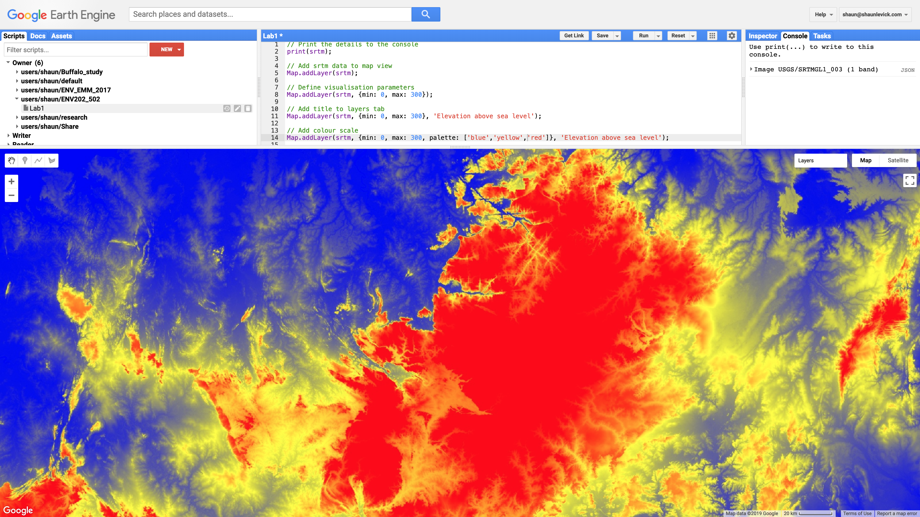
• If you would like to experiment with different colour combinations, you can play with colour palettes as per the example below:

Map.addLayer(srtm, {min: 0, max: 300, palette: ['blue', 'yellow', 'red']}, 'Elevation above sea level');

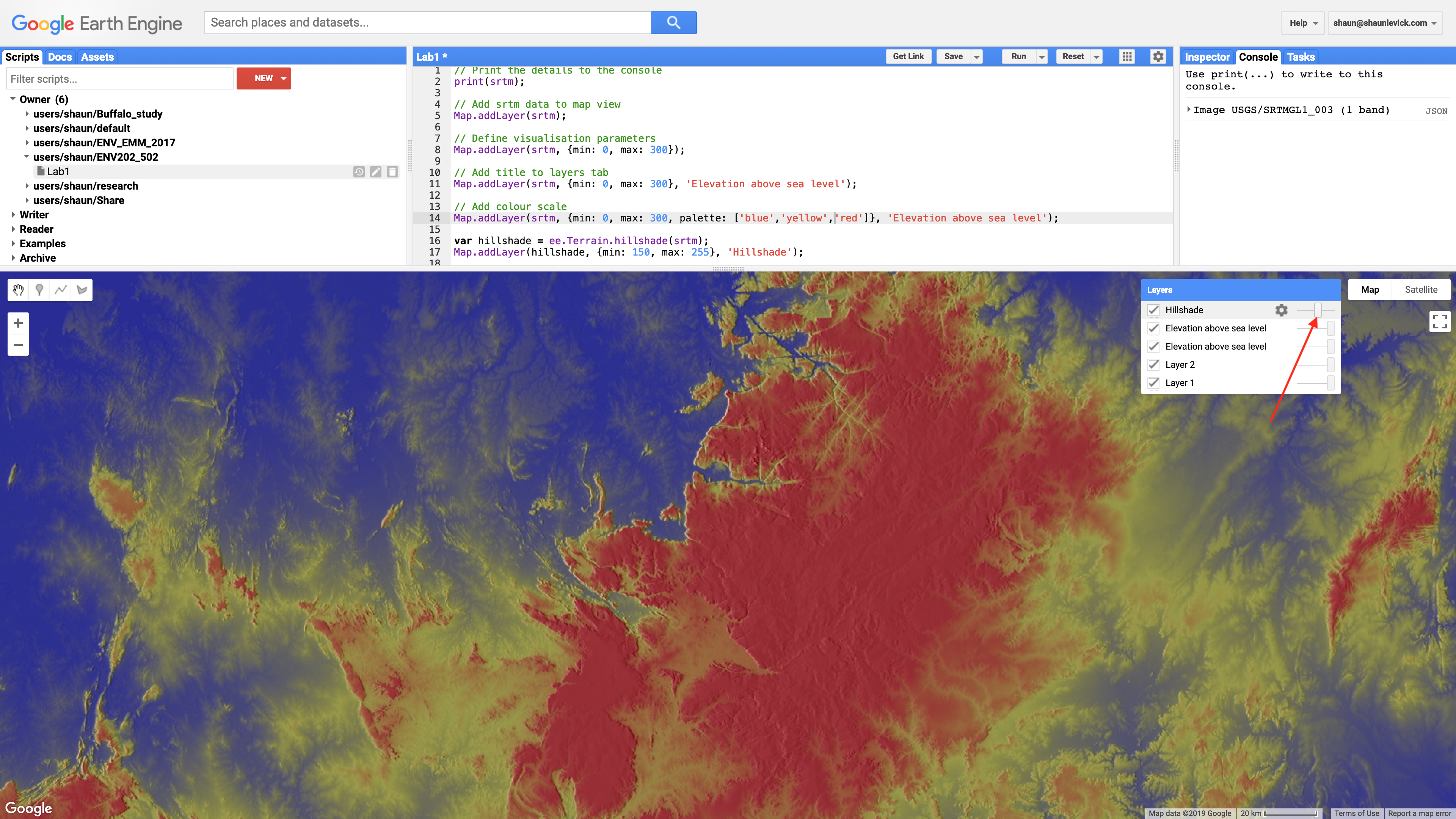
Hillshading and slope

• For better visualisation we can create a hillshade view of the elevation data. Remember you can use the Layer transparency options to create draped images for colourised hillshades.

var hillshade = ee.Terrain.hillshade(srtm);
Map.addLayer(hillshade, {min: 150, max:255}, 'Hillshade');

• Slope works in a similar way:

var slope = ee.Terrain.slope(srtm);
Map.addLayer(slope, {min: 0, max: 20}, 'Slope')

Thank you

I hope you found that useful. A recorded video of this tutorial can be found on my YouTube Channel's Introduction to Remote Sensing of the Environment Playlist and on my lab website GEARS.

Kind regards, Shaun R Levick